Abhishek Goel

Aug 8, 20207 min read

Markov Chains - Modelling and Simulation in R

In the previous post, we explored Markov chains in R. In this post, we extend the topic further by introducing "markovchains" package in R. We will also see how to model and simulate Markov chains in R.

"markovchain" package

The package contains classes and method to create and manage (plot, print, export for example) discrete-time Markov chains. In addition, it provides functions to perform statistical (fitting and drawing random variates) and probabilistic analysis - Package Documentation

We will now be using markovchain package to easily work with discrete-time Markov chains in R. The package provides simple functions to create and plot transition probability matrix and find steady states, absorbing states, and many more things.

install.packages("markovchain")
#load the package using library command
library(markovchain)

It is recommended to install the package diagram (it provides an efficient way of plotting transition graphs in R) before proceeding further.

install.packages("diagram")
#load the package using library command
library(diagram)

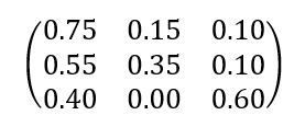
As an example, consider an insurance company providing unemployment insurance. We consider a Markov chain with three states: Employed (Emp), Unemployed(claiming benefit) (Unemp) and Inactive in the labour force (Inactive), measured at the end of each month.

Suppose the transition matrix, with the states in the order given above, is:

In order to set up the one‐step transition probability matrix for this process in R, we first create a vector of names of the states.

EmpStates <- c("Emp", "Unemp", "Inactive")

We then use the matrix function to set up this matrix in R. The byrow = TRUE argument tells R to input data values in the matrix by row.

Trans_Matrix <- matrix(c(0.75, 0.15, 0.10,
0.55, 0.35, 0.10, 
0.40, 0.00, 0.60), 
nrow = 3, byrow = TRUE)

Trans_Matrix
     [,1] [,2] [,3]
[1,] 0.75 0.15  0.1
[2,] 0.55 0.35  0.1
[3,] 0.40 0.00  0.6

We use the new function to define a Markov chain object in R:

mcEmpStatus <- new("markovchain", states = EmpStates, transitionMatrix = Trans_Matrix, name = "Employment Status")

The first argument "markovchain" specifies the class of the object we are creating, the second argument states take the vector of the names of the states, the third argument transitionMatrix takes the transition matrix, and the last argument name defines the name of our Markov chain.

mcEmpStatus
Employment Status 
 A  3 - dimensional discrete Markov Chain defined by the following states: 
 Emp, Unemp, Inactive 
 The transition matrix  (by rows)  is defined as follows: 
          Emp Unemp Inactive
Emp      0.75  0.15      0.1
Unemp    0.55  0.35      0.1
Inactive 0.40  0.00      0.6

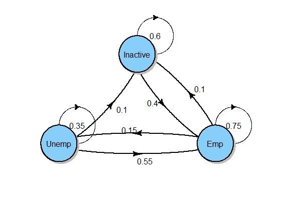
Let's plot the transition graph for our matrix! We do this by using the plot function and package diagram.

plot(mcEmpStatus, package = "diagram")

Neat and clean!

When creating a Markov chain using markovchain package, it gives us additional advantage of no longer multiplying the transition probability matrix successively many times or creating a function to calculate the n-step transition probability matrix. We can do this easily now with our Markov chain mcEmpStatus by simply raising it to the power n.

Suppose the process begins in state Emp. To see the probability distribution after 3 and 6 months, we use:

InitialState <- c(1,0,0)
After3Months <- InitialState * mcEmpStatus^3
After3Months
        Emp  Unemp Inactive
[1,] 0.6645 0.1605    0.175

After 6 months the probabilities are:

After6Months = InitialState * mcEmpStatus^6
After6Months
           Emp     Unemp Inactive
[1,] 0.6515785 0.1515465 0.196875

How easy was that!

Some useful functions of package "markovchain"

states() - This method returns the states of a Markov chain.
dim() - returns the dimensions of a Markov chain.
name() - returns the name of a Markov chain.
transitionProbability() - returns one-step transition probabilities of a Markov chain.
absorbingStates() - specifies the number of absorbing states in a Markov chain.
steadyStates() - returns steady state distribution of a Markov chain.
is.accessible() - This function verifies if a state is reachable from another (not necessarily in one-step).
is.irreducible() - This function verifies if a Markov chain is irreducible or not.
period() - determines periodicity of a Markov Chain.
summary() - provides summary of a Markov chain.
conditionalDistribution() - given a current state i it returns one-step transition probabilities of a Markov chain.

Let's run the functions one-by-one on the Markov chain mcEmpStatus.

states(mcEmpStatus)
[1] "Emp"      "Unemp"    "Inactive"

dim(mcEmpStatus)
[1] 3

name(mcEmpStatus)
[1] "Employment Status"

The transitionProbability function returns the one-step transition probabilities of a Markov chain. Let's calculate the one-step transition probability from state "Emp" to "Unemp".

transitionProbability(mcEmpStatus, t0 = "Emp", t1 = "Unemp")
[1] 0.15

The function absorbingStates specifies the number of absorbing states in the Markov chain. Here the output is character(0) which means there is no absorbing state in the Markov chain mcEmpStatus.

absorbingStates(mcEmpStatus)
character(0)

The function steadyStates returns the steady-state distribution (long-term stationary distribution) of a Markov chain.

steadyStates(mcEmpStatus)
      Emp Unemp Inactive
[1,] 0.65  0.15      0.2

The function is.accessible verifies if a state is reachable from another (not necessarily in one-step).

is.accessible(mcEmpStatus, from = "Inactive", to = "Emp")
[1] TRUE

Here the output TRUE indicates that the transition is possible from "Inactive" state to "Emp" state. The function below checks whether a Markov chain is irreducible or not.

is.irreducible(mcEmpStatus)
[1] TRUE

The function period determines the periodicity of a Markov Chain. The output below indicates that the Markov chain has a period of 1.

period(mcEmpStatus)
[1] 1

The most useful function summary provides a summary of a Markov chain by indicating the states, irreducibility, and absorbing states.

summary(mcEmpStatus)
Employment Status  Markov chain that is composed by: 
Closed classes: 
Emp Unemp Inactive 
Recurrent classes: 
{Emp,Unemp,Inactive}
Transient classes: 
NONE 
The Markov chain is irreducible 
The absorbing states are: NONE

The function conditionalDistribution returns one-step transition probabilities of a Markov chain given a current state i.

conditionalDistribution(mcEmpStatus, "Unemp")
     Emp    Unemp Inactive 
    0.55     0.35     0.10

Simulating a Markov chain

Markov chains are widely applied in the field of actuarial science. Two classical applications are policyholders’ distribution in Motor insurance and health insurance pricing and reserving.

Many stochastic processes used for modelling in insurance are Markovian, and this behaviour makes it easy to simulate Markov chains from them.

Simulating a Markov chain in R is quite straightforward using the function rmarkovchain.

Let's generate 15 years (180 months) of employment states according to mcEmpStatus Markov chain. We use set.seed for reproducible result and start with an initial state of "Emp".

set.seed(66)
REmpStatus <- rmarkovchain(180, mcEmpStatus, t0 = "Emp")
REmpStatus[1:30]
 [1] "Inactive" "Emp" "Emp"
 [4] "Emp" "Emp" "Emp"
 [7] "Emp" "Unemp" "Emp"
 [10] "Inactive" "Inactive"
 [12] "Inactive" "Inactive"
 [14] "Emp" "Unemp" "Emp"
 [17] "Emp" "Emp" "Emp"
 [20] "Emp" "Emp" "Emp"
 [23] "Emp" "Emp" "Emp"
 [26] "Emp" "Emp" "Unemp"
 [29] "Emp" "Emp"

Here we printed only the first 30 values (i.e. simulated states for first 30 months).

Note: Here the initial state "Emp" is not included in the simulated values. By this, we mean that X0 = "Emp" is not included in the result and the process starts at X1 which is "Inactive" as according to the simulated states. However, to include the initial state we can use an additional argument of include.t0 = TRUE in the function.

Modelling using Markov chains

In this section, we will try to fit a Markov chain to a set of observations. The Markov model must be fitted by first estimating the transition probabilities pij.

Estimating transition probabilities

Let's denote the observations by x1, x2,....., xn and define:

ni as the observed number of transitions from state i, and
nij as the observed number of transitions from state i to j.

Also,

The estimate of the transition probabilities pij is given as:

There are four methods to estimate transition probabilities in R: maximum likelihood, maximum likelihood with Laplace smoothing, Bootstrap approach, maximum a posteriori. However, we will only be using the default method (maximum likelihood) for our purpose.

We will be using the simulated values from mcEmpStatus Markov chain as a set of observations to which we will be fitting the Markov chain. This is done using the markovchainFit function from the markovchain package.

EmpFittedMLE <- markovchainFit(data = REmpStatus, method = "mle", name = "Employment Status")

We can then extract the estimate and standard error of the probability transition matrix as follows:

EmpFittedMLE$estimate
Employment Status 
 A  3 - dimensional discrete Markov Chain defined by the following states: 
 Emp, Inactive, Unemp 
 The transition matrix  (by rows)  is defined as follows: 
         Emp   Inactive  Unemp
Emp      0.81955 0.08271 0.09774
Inactive 0.46875 0.53125 0.00000
Unemp    0.71430 0.21430 0.07143

EmpFittedMLE$standardError
         Emp   Inactive  Unemp
Emp      0.07850 0.02494 0.02711
Inactive 0.12103 0.12885 0.00000
Unemp    0.22588 0.12372 0.07143

We can also only print the estimated transition probability matrix as follows:

EmpFittedMLE$estimate@transitionMatrix
         Emp   Inactive  Unemp
Emp      0.81955 0.08271 0.09774
Inactive 0.46875 0.53125 0.00000
Unemp    0.71430 0.21430 0.07143

There's also a function named createSequenceMatrix that returns the raw count transition matrix i.e. matrix of nij values (the observed number of transitions from state i to j).

createSequenceMatrix(stringchar = REmpStatus)
         Emp Inactive Unemp
Emp      109       11    13
Inactive  15       17     0
Unemp     10        3     1

A special function, multinomialConfidenceIntervals, can be used to obtain multinomial wise confidence intervals.

multinomialConfidenceIntervals(transitionMatrix = EmpFittedMLE$estimate@transitionMatrix, countsTransitionMatrix = createSequenceMatrix(REmpStatus), confidencelevel = 0.95)
$confidenceLevel
[1] 0.95

$lowerEndpointMatrix
         Emp  Inactive Unemp
Emp      0.7670 0.0301 0.0451
Inactive 0.3125 0.3750 0.0000
Unemp    0.5714 0.0714 0.0000

$upperEndpointMatrix
         Emp  Inactive Unemp
Emp      0.8870 0.1501 0.1651
Inactive 0.6491 0.7116 0.1804
Unemp    0.9835 0.4835 0.3407

Prediction (n-step ahead)

The n-step forward predictions can be obtained using the predict function.

The 3-months forward predictions from markovchain object can be generated as follows, assuming that the last two months were respectively “Unemp” and "Emp”.

predict(object = EmpFittedMLE$estimate, newdata = c("Unemp", "Emp"), n.ahead = 3)
[1] "Emp" "Emp" "Emp"

The next step is to check whether the Markov property holds or not. It is generally done using triplets test.

Assessing the Markov property

The verifyMarkovProperty function verifies whether the Markov property holds for the given chain. The function performs a triplets test on the chain.

Triplets test

Let nijk denote the number of observed transitions from state i to j to k. If the Markov property holds we expect nijk to follow a binomial distribution with parameters nij and pjk. The chi-square goodness-fit-test is used to test this assumption. The test statistic is given as:

The null hypothesis is:

H0: the process has the Markov property

The alternative hypothesis is:

H1: the process does not have the Markov property

Under the null hypothesis, Nijk ~ Binomial(nij, pjk).

We perform the test on the simulated values of the Markov chain mcEmpStatus.

verifyMarkovProperty(REmpStatus)
Testing markovianity property on given data sequence
Chi - square statistic is: 1.248648 
Degrees of freedom are: 27 
And corresponding p-value is: 1 
Warning message:
In verifyMarkovProperty(REmpStatus) :
The accuracy of the statistical inference functions has been questioned. It will be thoroughly investigated in future versions of the package.

Since the p-value shown is above 0.05, we do not reject the null hypothesis that the sequence follows the Markov property. Well, this is obvious in this case since we are assessing the fit on the simulated values from a Markov chain.

Note: However, as mentioned in the warning message the accuracy of the statistical inference functions has been questioned.

Let's consider a sample sequence:

sample_seq <- c(1,3,2,2,1,3,3,2,3,1,2,3,2,1,1,2,2,1,3,3)
verifyMarkovProperty(sample_seq)
Testing markovianity property on given data sequence
Chi - square statistic is: 8.277778 
Degrees of freedom are: 27 
And corresponding p-value is: 0.9997963

Since the p-value is greater than 0.05, we do not reject the null hypothesis.

Thank you for reading the post. I hope you enjoyed it! Do let me know in the comments if you enjoyed reading this post. I would be very grateful if you’d help it spread by sharing it with your friends and network. Thank you!

—Abhishek Goel

I am currently an actuarial student and the above blog is to the best of my knowledge. I do not claim to be expert in the field. I am just sharing my learning with others and this is an effort to help other students learn R. Your feedback and suggestions are welcomed.

References